The instructions on this page guide you through the process of creating a nebula using Chaos Phoenix 4 and V-Ray GPU.
Overview
This is an Intermediate Level tutorial. Even though no previous knowledge of Phoenix is required to follow along, re-purposing the setup shown here to another shot may require a deeper understanding of the host platform's tools, and some modifications of the simulation settings.
In this tutorial, we are going to show you how to create a nebula with Phoenix. Since a nebula is a giant cloud of dust and gas in space, we will simulate it as smoke and then we will add lights to give it the appearance of a nebula. After simulating with a single Simulator, we will duplicate it into five additional instances, to have six simulation grids in total.
For better rendering performance, we will render the scene using V-Ray GPU.
The simulation requires using Phoenix 4.41.00, and V-Ray 5 Update 1 for Maya 2018 at least. You can download official Phoenix and V-Ray from https://download.chaos.com. If you notice a major difference between the results shown here and the behavior of your setup, please reach us using the Support Form.
The Download button below provides you with an archive containing the start and end scenes.
Units Setup
Scale is crucial for the behavior of any simulation. The real-world size of the Simulator in units is important for the simulation dynamics.
Large scale simulations appear to move slower, while mid-to-small scale simulations have lots of vigorous movements.
As the focus of this tutorial is a large-scale simulation, setting the units to Meters is a reasonable choice.
Go to Windows → Settings/Preferences → Preferences and then click on Settings. Underneath the Working Units, change the Linear dropdown to meter and click Save.
The Phoenix solver is not affected by how you choose to view the Maya Working Units - it is just a matter of convenience.

Note that when you create your Simulator, you must check the Grid rollout where the real-world extents of the Simulator are shown.
If the size of the Simulator in the scene cannot be changed, you can cheat the solver into working as if the scale is larger or smaller, by changing the Scene Scale option in the Grid rollout.

Color Management Settings
We also want to make sure our Color Management preferences are set to work properly. If you're using a version of Maya 2018, 2019 or 2020, you can leave the Color Management settings at the default values, which should be in sRGB rendering space.
If you're using Maya 2022 or later, head to the next step below.
You can see the Color Management default settings on the right for Maya 2018, which will be the basis for the settings used in this tutorial.

If you're using Maya 2022, the Color Management settings have been changed to ACEScg by default.
We need to switch them to sRGB settings, so that the render results in this tutorial remain consistent with earlier versions of Maya as well.
In the Color Management section, change the Rendering Space to scene-linear Rec.709-sRGB.
Set the Display to sRGB.
Set the View to Raw.
This way, Color Correction presets that have been provided with the Nebula project file will work as expected. We'll take a look at them later on in the tutorial.

Scene Layout
In this tutorial, we will create a single simulation for the initial setup and then duplicate it five times as an instance for the final setup.
Initial scene setup consists of the following elements:
- A deformed Torus Knot geometry that is used for the smoke source.
- Phoenix Fluid Simulator (PhoenixFDSim1).
- Phoenix Fire/Smoke Source (PhoenixFDSrc1) emitting Smoke from the Torus Knot geometry.
- VRayLightSphere1 light for lighting.
- Camera1 for look-development rendering.
- Phoenix Turbulence (PhoenixFDTurb1) for adding variation to the Smoke's motion.

The final scene setup consists of the following elements:
- An original Phoenix Fluid Simulator (PhoenixFDSim1) + five instances (PhoenixFDSim2 - PhoenixFDSim6).
- Three additional VRayLightSpheres (VRayLightSphere2 - 4) for lighting.
- A Semi-circular Curve, serving as a camera animation path.
- Camera2 for the final animation render. Camera2 is path constrained to the Semi-circular Curve.
- An nParticle grid used to replicate stars.
In the "Nebula_Maya2018_Start.ma" scene, the VRayLightSphere2-4 lights are turned off and hidden, and the nParticle grid is hidden as well.

If you're using Maya 2018 or an earlier version, note that you will need to adjust a setting in order for the Camera2 animation to function as expected.
Simply set the Maya Preferences → Animation → Evaluation mode to DG, and this will produce the proper behavior and results for Camera2's animation path.
If the Evaluation mode is not set to DG for Maya 2018 and earlier, your camera animation may experience an offset frame during playback and rendering.
Note that this issue does not apply to later versions of Maya, such as Maya 2019, 2020 and 2022.

The geometry used for the smoke emission is a custom Torus Knot, which you can feel free to use in your scene as well. It was deformed to give it a more organic look.
You can replace the Torus Knot with any other geometry you like, e.g. a donut geometry. The emitter geometry determines the initial shape of the nebula.
In the later stages of the tutorial, we will blow away the nebula smoke using Phoenix Turbulence to add more variation, but the geometry still plays an important role in affecting the final appearance of the nebula.
Note that the Torus Knot is set to be non-renderable, from its Render Stats options in Maya. This way, when we render we'll only see the results of the nebula, and the geometry will not be visible.

Lights, Cameras and Environment
In this tutorial we have many steps to follow. To keep it concise, let's focus only on the Phoenix related steps. Feel free to use the camera and light settings in the provided sample scene.
For your reference, below you can find the light, camera and VrayLightMtl settings for the nParticles.
Lights Settings
Final details for the four VRayLightSphere lights.
*Note: For preview purposes, we will initially set the VRayLightSphere1 Multiplier to 10, until we enable the rest of the lights later on and lower its multiplier.
| Position | Multiplier | RGB Color | Radius | |
|---|---|---|---|---|
| VRayLightSphere1 | 2.5, 12.0, 0.0 | 10* (4.0 at finish) | 146, 168, 239 | 4.0 |
| VRayLightSphere2 | -30.0, 33.0, 1.0 | 6.0 | 23, 81, 230 | 2.0 |
| VRayLightSphere3 | -32.5, 8.5, -7.0 | 0.4 | 47, 89, 224 | 2.0 |
| VRayLightSphere4 | 38.7, 12.3, 1.0 | 1.0 | 83, 132, 230 | 8.0 |
In the Options for all of the VRayLightSphere lights, enable the invisible checkbox, so that we do not see the light source directly.

nParticle Settings
An nParticle system is used for the stars. To mimic stars, a VRayLightMtl is applied to it. The Color is set to RGB (255, 255, 255) and the Color Multiplier to 100.0.


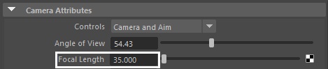
Camera Settings
We have two cameras in the scene, both set to the Camera and Aim control mode. Camera1 is static, and Camera2 is moving along the Semi-circular Curve.
Camera1 has a starting position that we will later update to a new position. For now, we want it to focus on the main Nebula simulator, so we get a nice preview as we work.
The starting position of Camera1:
Focal Length is set to 35.0.
Camera Aperture (mm) is set to 36.0.
The exact position of Camera1 is XYZ: [ -31.3, 10, -65.5 ].
The exact position of the Camera1_aim is XYZ: [ -0.9, 11.4, -5.7 ].


Camera2:
Focal Length is set to 45.0.
Camera Aperture (mm) is set to 36.0.
The exact starting position of Camera2 is XYZ: [ -21.0, 38.1, -125.6 ].
The exact position of the Camera2_aim is XYZ: [ 0.1, 19.2, 1.3 ].
Circular Curve:
Camera2 is also path constrained to a Semi-circular Curve.
The exact position of the Semi-circular Curve is XYZ: [ -10.5, 38.1, 39.4 ].
Its rotation is set to XYZ: [ 0, 4.5, 0 ].


Camera2 motion path:
From frames 0 to 72, the Camera2 motionPath2_uValue is constricted so that the camera is animated along a certain section of the curve. The value at frame 0 is set to 0.0044, and frame 72 is set to 0.00487. The InTan Type and OutTan Type are both set to Linear.

Phoenix Simulation
Go to the menu for PhoenixFD → Create → 3D Simulator.
The exact position of the Phoenix Simulator in the scene is XYZ: [ -2.0, -0.17, 0.0 ].
Open the Grid rollout and set the following values:
- Scene Scale: 1.0.
- Cell Size: 0.086 m.
- Size XYZ: [ 363, 261, 371 ] - we keep the Simulator size small enough to cover only the emission geometry.

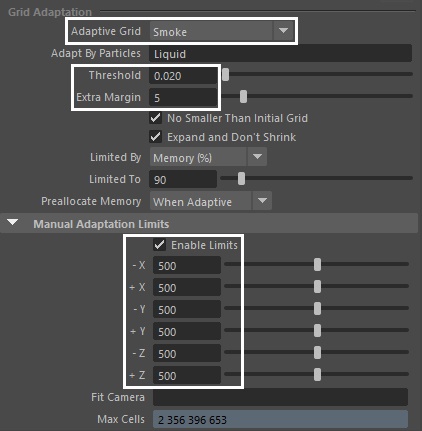
- Adaptive Grid: Smoke - the Adaptive Grid algorithm allows the bounding box of the simulation to dynamically expand on-demand.
- Set a Threshold of 0.02, so that the Simulator expands when the Cells near the corners of the simulation bounding box reach a Smoke value of 0.02 or greater;
- Extra Margin: 5.
- The Extra Margin option is useful when the Adaptive Grid algorithm is unable to expand fast enough to accommodate quick movement in the simulation (e.g. an explosion). The Extra Margin attempts to remedy this by expanding the grid preemptively with the specified number of voxels on each side.
- Enable Expand and Don't Shrink - this way the Adaptive grid will not contract back when there is very thin smoke at the borders of the grid.
- In the Manual Adaptation Limits rollout, check on Enable Limits and set the values to: X: (500, 500), Y: (500, 500), Z: (500, 500) - to save memory and simulation time by limiting the Maximum Size of the simulation grid.
Later in the tutorial we are going to duplicate the Simulator a few times and scatter the instances in the scene.
As we don't want to see any seams where the Simulators overlap, using the Adaptive Grid with the Enable Limits option will prevent us from creating a cropped volume at the Simulator's boundary.
Select the Phoenix Simulator → Output rollout and enable the output of Grid Smoke, Grid Wavelet, and Grid Velocity Channels.
Any channel that you intend to use after the simulation is complete, needs to be cached to disk. For example:
- Grid Velocity is required at render time for Motion Blur.
- Grid Temperature/Liquid is usually used at render time to generate Fire or Liquid.
- Grid Wavelet is used for Wavelet turbulence when performing a Resimulation.

Adding Fire/Smoke Sources
Create a Phoenix Fire/Smoke Source in the scene by going to: PhoenixFD → Create → PHXSource.
Select the TorusKnot geometry as the emitter, and then press CTRL+LMB and click on PhoenixFDSrc1, so that both the Torus and PHXSource are selected. Then, press the Add Selected Objects button in the PhoenixFDSrc1 attributes.


For the PhoenixFDSrc1:
Set the Emit Mode to Surface Force, Discharge to 1.0 and Smoke to 4.0.
Disable the Temperature option.
We increase the smoke amount to 4.0, so that the nebula appears more opaque in its core.

In the Simulator → Simulation rollout, disable Use Timeline Stop Frame, and set the Custom Stop Frame to 30.
The Use Timeline Stop Frame checkbox needs to be disabled so that we can modify the parameter value below.

Here is a Preview Animation of the simulation up to this step. It looks a bit dull now and does not yet resemble anything like a nebula.
To enable the GPU Preview as seen in the video, select the Phoenix Simulator → Preview rollout → GPU Shade Preview → Enable GPU Preview.
At this step, the nebula appears blue because the color of the VRayLightSphere1 is set to a light blue color.
Adding Phoenix Turbulence
Go to Phoenix FD → Create → Turbulence.
Position to XYZ: [ -2.5, 14.0, 9.0 ].
Set the Strength to 350.0 and the Size (units) to 30.0.
Reduce the Fractal Depth to 1.
Set the Decay type to Inverse square.
Then go to the Phoenix Simulator and run the simulation again.
The position of the Phoenix Turbulence does affect the result of the simulation. If you did not set the exact position as mentioned above, you probably won't get the same results.

Here is a Viewport Preview showing the result of the simulation so far.
Input
Once the simulation is complete, go to the Phoenix Simulator → Input rollout.
For this tutorial we need only a static nebula, switch the Time Bend Controls → Playback Mode to Cache Index. Set the Direct Cache Index to 29.0.
You can set the Direct Cache Index to any other frame you like. Different frames create different characteristics for the nebula. Later frames will have a more dispersed and smoky look, due to the Turbulence force.

Volumetric Shading - Smoke Color
Go to the Phoenix Simulator → Rendering rollout.
Drop down the Fire rollout, and set the Based on option to Disabled.

For the Smoke Color rollout, set the Based on option to Smoke. Adjust the color gradient as shown in the image.
The Color gradient is set to blue-pink-red-purple-black, representing the smoke color at different smoke densities, from sparsest to densest. Feel free to customize the color gradient according to your preference.

Smoke Opacity
For the Smoke Opacity rollout, set the Based on option to Smoke.

Then, adjust the Opacity curve below, as shown in the image.

Alternatively, you can simply load up a Rendering Preset using the Nebula_Rendering_Preset.mel file, that is provided with the sample scene.
Note that there is an additional .mel preset file as well, which contains additional tweaks that we'll create near the end of the tutorial.

GPU Rendering
Since we are going to render a very heavy volumetric scene, we will use V-Ray GPU as our renderer.
Since Global Illumination does not contribute a lot to this scene, let's disable the GI in the Render Settings → GI tab.

For preview purposes, let's make sure that only the VRayLightSphere1 is enabled. Set its Intensity multiplier to 10 for now, until we enable the other lights later on.

Here is a test rendering up to this step.
For test rendering, we set the Sampler type to Progressive and set the Maximum render time (min) to 10.0 for the V-Ray GPU renderer. You can adjust the time limit depending on your hardware.

If we move the VRayLightSphere1 a little behind the nebula, or move it towards the camera, notice how the appearance of the nebula dramatically changes by simply changing the light's position.
Here are a few comparison images from left to right, with different light positions: Behind (2.5, 12, 12), Center (2.5, 12, 0), Front (2.5, 12, -12).

Buffered Conservation
Select the Phoenix Simulator. Disable the Gravity, since a nebula supposedly forms in outer space.
Note that since we simulated without the Temperature channel, there is no difference in the simulation results with or without gravity.

Change the Conservation Method to Buffered, and set the Quality to 40.
Set the Steps Per Frame to 2.
The Buffered method has the weakest conservation strength and shortest range, but produces nice details. For in-depth information, check the Conservation documentation.

Here is a test render up to this step. We can see a better pattern formation, compared to the results with the default Dynamics settings.

Resimulation
Open the Phoenix Simulator → Resimulation rollout and enable Grid Resimulation.
Note that when you enable Resimulation, Phoenix will try to read the cache files for preview and rendering from the Resimulation Output Path, instead of the 'regular' Output. Don't worry if the Viewport goes blank and the preview disappears - you can always go back to the original cache files by disabling the Resimulate checkbox.
Set the Amplify Resolution to 0.2. This parameter is used to increase the resolution of the grid during the Resimulation process.
Set the Amplify Method to Wavelet Nice and Wavelet Strength to 1.0.
Press Simulator → Simulation rollout → Start to begin the Resimulation.
We set the Wavelet Strength to 1.0 instead of 3 (default value), because we want to add details to our base simulation, without overdoing it.
You can set the Amplify Resolution to an even higher value to get a more detailed result.

Here is a test render up to this step. As you can see, after the Resimulation, we got more details in the smoky cloud, while maintaining the overall pattern formation from the base simulation.

Simulator Duplication & Positioning
With the Phoenix Simulator selected, go to Edit → Duplicate Special and click the menu to see more options. Change the Geometry type to Instance, and set the Translate value for X to 100. Then set the Number of Copies to 5 and press Duplicate Special.
Now we have six Phoenix Simulators in total (PhoenixFDFire001~006).
The benefit of the Duplicate Special method we mentioned above is that the Instanced Simulators won't be created in the same position. This way it will be easier for us to select them in the viewport.

Next we will move and rotate the Simulator instances in the scene, and arrange them to match the screenshot on the right.
Since all six Simulators are exactly the same, we will have to rotate them in order to avoid any obvious repetitive patterns.

Rotate the PhoenixFDSim1 simulator -20 degrees on the Y axis.
Now we will have a more noticeable gap in the center of the nebula, for V-RayLightSphere1 to shine through. This will help to create a more pleasing composition, in tandem with the additional duplicated nebulas.
Also rotate the Torus Knot geometry -20 degrees on the Y axis as well. That way if you decide to simulate again later, the Torus Knot will already be rotated.

The table on the right provides the exact location and rotation of each Simulator instance. You can customize the transformation of each Simulator according to your preference.
| Position | Rotation |
|---|---|---|
PhoenixFDSim1 | -2, -0.17, 0 | 0, -20, 0 |
PhoenixFDSim2 | 38.5, 0, -11.5 | 0, 125, 0 |
PhoenixFDSim3 | -37, 0, -3 | 0, -136, 0 |
PhoenixFDSim4 | -3, 50.5, 0 | 121.5, 0, 0 |
PhoenixFDSim5 | -25, 35.5, -3 | 87.5, -103.5, 0 |
PhoenixFDSim6 | 41.5, 54, 0 | 156, -58, 0 |
Final Lighting Setup
To make the image more interesting, turn on the other three VRayLightSphere lights (VRayLightSphere2 - 4) in the scene.

Let's also move the Camera1 and Camera1_aim, so that we can get a better view of the duplicated Nebulas.
Set the Camera1 Position to XYZ: [-53.2, 20.5, -94.0] and the Camera1_aim Position to XYZ: [1.7, 20.5, -2.1].
Also, set Camera1 the Focal Length to 40.

Here is a test render up to this step.
So far so good, but the VRayLightSphere1 is too bright relative to the other lights, so let's bring that down a bit.
Lower the Intensity multiplier to 4.0 for the VRayLightSphere1, so that it is more balanced with the rest of the lights we just enabled.

Now both the lighting and volumetric simulation are ready for rendering. We'll then do some Color Corrections in the V-Ray Frame Buffer, to bring out the detail and make the image more dynamic.
Also, to render out the stars, make sure to unhide the nParticles in the scene, and then do a render and proceed to the next step.

V-Ray Frame Buffer & Color Corrections
Open the V-Ray Frame Buffer and use the Create Layer icon to add layers for Filmic Tonemapping, Color Balance, Curves, White Balance and Lens Effects.
Using V-Ray 5 as a render engine gives us the advantage of using Filmic tonemapping directly in the new VFB. However, if you are using an older version of V-Ray for Maya, you can get a similar effect by using a proper LUT.
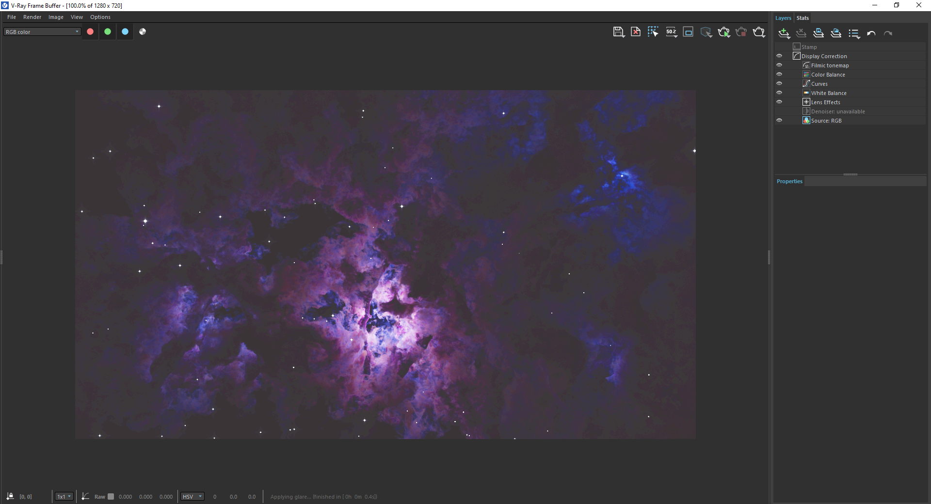
The final image is rendered using the V-Ray Frame Buffer with the color corrections & post-effects set to:
Filmic Tonemap:
- Blending: Overwrite, 1.000;
- Tone mapping space: Linear sRGB;
- Type: Hable;
- Log space: disabled;
- Gamma: 1.000;
- Shoulder strength: 0.670;
- Linear strength: 0.070;
- Linear angle: 0.490;
- Toe strength: 0.270;
- White point: 7.880.
Color Balance:
- Blending: Overwrite, 1.000;
- Selection mode: All;
- Cyan - Red: -0.093;
- Magenta - Green: -0.020;
- Yellow - Blue: -0.082.
Curves:
- Adjust it to an S-shape curve as shown in the screenshot.
- Blending: Overwrite, 1.000;
- 1st Coordinate: [-0.00746, 0.00862];
- 2nd Coordinate: [1.000, 1.004].
White Balance:
- Blending: Overwrite, 1.000;
- Temperature: 6519.126;
- Magenta - Green tint: -0.040;
- Color Tint (RGB): [1.000, 1.000, 1.000].
Lens Effects:
- Opacity: 1.000;
- Enable bloom/glare;
- Size: 11.110;
- Intensity: 0.050;
- Bloom: 0.500;
- Threshold: 0.570;
- Rotation: 0.000;
- Saturation: 1.000;
- Enable Hardware accelerated;
- Enable Cold/Warm;
- Enable Interactive;
- For Aperture Shape:
- Enable Blades;
- Sides: 4;
- Blade rotation: 45.000;
- Streak blur: 0.200;
- Everything below in the Lens Effects is disabled.
The Filmic tonemap allows you to simulate the film response to light within the VFB.
Feel free to use other values for the post effects, depending on your preferences.


Alternatively, you can simply load up the Color Corrections Preset from the Nebula_VFB_CC.vfbl file that is provided in the sample scene.

Smoke Color Absorption
As a final step and to further enhance the realism of the nebula, let's also introduce some Color Absorption, which controls the color of the volumetric shadows and the tint for the objects seen through the volume. Select the Phoenix Simulator, go to Rendering → Smoke Opacity.
Set the Absorption Constant Color to a green RGB (91, 96, 55).
The absorption color here is basically complimentary to the purple color of the nebula. However, you can feel free to choose another color.
Note that when the Constant Color is set to a darker color, it will appear more opaque (dense). Meanwhile, brighter colors make the volume more transparent. You can play with this parameter to find something that suits your preference.

Alternatively, you can load in the final preset file Nebula_Rendering_Preset_02.mel which contains the final Absorption Constant Color as well.

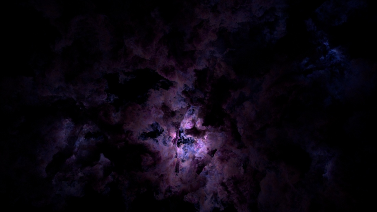
Final Results
Here is the final rendered image with the Absorption Color and Color Corrections we set up earlier.

Tweaking the Absorption Color setting brings out additional details and colors in the nebula, especially around the brighter areas.


And here is the final rendered animation result.